One-parameter family of functions

Here’s a fun paper to read: Real numbers, data science and chaos: How to fit any dataset with a single parameter. The premise of the paper is that “all the samples of any arbitrary data set can be reproduced by a simple differentiable equation”, namely, this one:

where is “learned” from the data set. And to illustrate this, they provide some examples along with their learned parameter.

The crazy part, they apply this to other types of data, including time series.

Of course, that doesn’t mean that you can use this to make any prediction or classification, etc. Quite the opposite, one of the goals of the authors is to warn against interpretations that come out of any machine learning model, and they do this beautifully and mention it in Section 3 of the paper. But let’s take a moment to understand what is the thing that they actually do?

If I’d asked you to create a one-parameter family of functions that “fits” any given data set what would you do? You might think of lines that pass through the origin. And then you might think, well, that doesn’t “fit” anything really, at best, it shows a trend in the data.

This is when I start explaining that by fitting I really mean just curve fitting, some function for which the sum of the vertical distances of the observed points from the curve is minimized. Without really any other assumptions, constraints, etc. The ideal one will have RMSE (root mean square error) zero. Something like this:

Here a reasonable person would explain that such a thing, even if possible, would not serve any real purpose, other than just connecting those dots. And that is what I’ve actually done there, I’ve connected the dots with line segments. But I’ll keep explaining that I’m really just interested in knowing if there is a family of functions that could do this for me, where suddenly a mathematically oriented person would point out that yeah, you can estimate it with a polynomial of large enough degree, right before someone pointing out that that’s not gonna be a “one-parameter” family though.

The thinking here is that high-degree polynomials will give you enough zeros, enough oscillations that then you could control by adjusting the coefficients of the polynomial. The fit is going to be awful for any practical purpose, but the RMSE will go to zero if you choose the degree large enough. OK, I’m not even going to attempt plotting one for the above data set, since it will fill the whole area with red lines, but here is one for a much smaller set just for your imagination:

Even though the polynomial idea was not that good (too many parameters) it points in a good direction (thanks the mathematically oriented person who suggested this). The reason a polynomial of high degree can do this is that it has many zeros (more than a line) and with coefficients, you can “tune” them to fit your data set well. Now that we don’t have the luxury of many coefficients, maybe we can use many zeros somehow?! So, what would you do, if you wanted to achieve many zeros with a function that doesn’t have many parameters? Yes, an oscillating function like would do.

Now, you probably need to space the zeros of the function so that they are not uniform, one idea could be to space them exponentially, that is, to use . this will introduce a lot more zeros in a limited domain and space them unevenly, the further you go, the more zeros:

We’re almost there, now if you just shrink or stretch the function horizontally, you might have a good chance of “fitting” many many data sets with really low RMSE. And in this very interesting paper, Laurent Boué does exactly that. Well, not exactly, there are a few more details to take care of the precision, and also it’s a so that the numbers are between zero and one, for simplicity I guess, or for being fancy, I don’t know. The is just a number that shrinks and stretches the function horizontally, and I think all of it could have been called the , but again for some computational reasons, or for the sake of being fancy, or something else, it was used like this. The catch here is that you need to reeeeeally fine-tune that to get what you want and to achieve this, they have to do the calculations with really high precision, and apparently, to be able to do that you need to do it in binary, with strings?! And at the end, what you have is a purely(?) mathematical hash function. Yes, you are not fitting or learning anything, to be honest, this is just an interesting hash function. Anyways, enjoy reading the paper, especially Section 3.

Mutually informing the cause?

Disclaimer: I’m not a statistician, and no, correlation does not mean causation. Also, I’m not a seismologist. And none of the followings are necessarily true. I’m just stretching my thoughts here!

To begin, read this and then take a look at this. Then come back and we’ll talk about something related.

Welcome back! OK, I don’t really want to talk about causality, I’m interested in the direction of the information flow. What do I mean by that? Let’s say there was an earthquake and two recordings of it are available from two different stations. Can we figure out which one is closer to the centre of the earthquake? Considering both stations use the same devices and the same settings, it should be the one that shows the signals first. Or, at least that’s my guess. Here is a very fake picture:

You’d guess the information is flowing from the station which made the top recording towards the one that made the bottom one. But in general, the signals are not gonna be this clear. So, let me try with another example:

One traditional way of detecting what we could detect with our eyes in the previous picture is to lag the second signal by samples and find the cross-correlation of the first signal with these lagged signals. Where the maximum occurs tells you which one received the information first, and by how much delay.

This detects the delay almost exactly where it is. And note that the correlation is positive here. Another way of comparing two signals is to compute their mutual information. If I do the same lagging and replace the correlation with mutual information I’ll get a picture like this:

And here also we can detect the delay with the same precision. There are some considerations that one needs to take into account. One is that the mutual information is less robust than correlation. Another thing is the calculation is much slower for hundreds of lagged signals. Also, one needs to bin the data to find their joint entropy before being able to compute the mutual information, and deciding about how to bin the data could become a problem on its own.

One more detail here is that this delay detection can be done when one of the signals are anti-correlated with the other one. For example, if I turn the second signal above upside down, then do the same analysis, I’ll find out the maximum happens the same way for the mutual information, but at the negatives for cross-correlation, since I’m finding the maximum of absolute values of them.

All that said, there are more established ways of looking at such data out there, and here are a few of them that for any practical purposes, you might wanna use those. The code to compute above examples and mutual entropy is on my GitHub.

Here I want to talk a little about the mutual information itself and how to compute it, along with details about joint entropy.

Entropy and joint entropy

Entropy of a probability distribution is defined to be

Now, let’s assume I have a vector of length . This vector could be a sampled signal. I could find a probability distribution of each number here, but most probably I’m going to end up with unique numbers in which means the probability of each of them is and then the entropy is simply the maximum possible entropy for a vector of this length, which is . OK, I’m implicitly saying

for any probability distribution of events. This means one can normalize entropy to be able to compare information of varying length. Also, a list of unique numbers will reach this maximum entropy.

That is, this doesn’t tell me anything about my signal. All of the entries of my signal are probably distinct. Hence, I need to bin my data in order to get a nontrivial probability distribution. Let’s say for the moment I decide to have 10 bins and put my data into those bins. Then I can count how many points are in each bin and that will give me a nontrivial probability distribution if I haven’t chosen my bins too small or too big. In order to do so in Matlab, I can decide what is the number of bins I want to have nbins and then

edgex = min(X):(max(X)-min(X))/nbins:max(X)+(max(X)-min(X))/nbins; % creat bins
edgey = min(Y):(max(Y)-min(Y))/nbins:max(Y)+(max(Y)-min(Y))/nbins; % creat bins
Xb = discretize(X,edgex); % bin X
Yb = discretize(Y,edgey); % bin Y

Here I’m adding an extra bin at the end to ensure the numbers in the top bin are accounted for. Then I can find the number of unique elements in Xb and Yb by looking at the third output of theunique() command and count how many of each unique number is there by the help of accumarray(), and its probability is the frequency divided by the number of unique numbers. The rest is plugging this information into the formula.

The joint entropy, then is to find the joint probability distribution of Xb and Yb, and then repeating the process. Here the joint probability distribution is computed by counting how many times each ordered pair has appeared in the list. for example if
Xb = [1, 1, 1, -1, -1, -1] and
Yb = [1, -1, 1, -1, 1, -1], then the ordered pair (1,1) appears exactly twice, in the first and third position. To make this example complete, the joint frequency distribution will look like this:
2    1
1    2
and then the joint probability distribution is that devided by 6 = 2+1+1+2 = length(Xb). The joint entropy is then

For eample, in the case of example above, it is

The joint entropy then has the property that

And finally, the mutual information is defined as

Then it is easy to see that the mutual information is always positive, and theoretically no less than . which means this mutual information can be normalized so that we can compare information of different lengths.

In the example above, the entropy of both X and Y here is 1, and their joint entropy is about 1.92, which leads to a mutual information of about 0.08. Their entropy tells me that optimally I need 1 bit to express each of them, and their joint entropy says optimally I’ll need less than 2 bits to be able to express both of them(?). But I’m not sure how does this exactly work! That is overall, about 0.08 of their information is overlapping and can be saved in communication.

I am interested in figuring out what is the maximum possible joint entropy and what pair or probability distributions yield it. Same thing for the mutual information. Also, when two signals have zero mutual information, or maximum mutual information, what does it say about them? What does it even mean? Share your thoughts 🙂

—

Most of my understanding of the topic came from this great post.

Many of the details I’ve learned through discussions with Aiden Huffman and Gabi Zeller.

If you treat a network like a dynamical system…

Let’s say we have a graph (i.e. network), and we want to cluster the vertices (nodes).  Here, think of the nodes as people, agents, oscillators, some dynamic being, and the edges… the edges tell you if these people are friends or enemies, and how much, they tell you if the agents want to collaborate with each other or not, they tell you if the oscillators attract each other or repel each other, and how much. This means we have a (signed weighted) network that can be treated as a dynamical system. One of the most famous and simple (nonlinear) dynamical systems that can model attraction/repulsion is the Kuramoto model. In simple terms, it says if you have oscillators and each of them is moving around the unit circle with a natural frequency while being attracted/repelled by other oscillators as strongly as , the derivative of its phase with respect to time (the angular velocity, the rate of change of its phase) is given by

The Kuramoto model

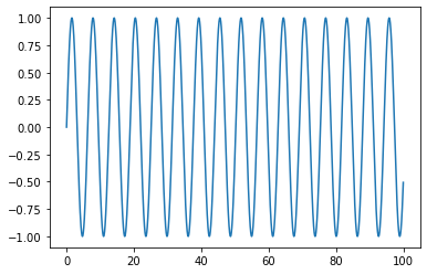
where , is called the coupling strength of the system. At the beginning when they are not coupled, their movement looks like this:

 

Five uncoupled oscillators with some natural frequencies

 

The order parameter, which is simply the length of the vector of the sum of their positions, will look like this:

There is no synchrony. But if we assume all of them attract each other, that is, if all , then they’ll start behaving like this:

 

Five coupled oscillators with some natural frequencies

 

They soon synchronize and stay “together”! The order parameter will look like this:

I’m not sure what those bumps towards the right end are, beginning of a chaos?

Anyways, the fact that all of them synced together tells me that the network is very well connected, and probably I don’t want to break it into clusters since there’s only one meaningful cluster out there.  But if I start with some network like this:

And run the model, I will end up with some final phases likeWhich, in turn, will be clustered as

This reveals the underlying clustering of my network. Matlab/Octave code for calculations can be found on my GitHub.

Balls, bins, and the Hungarian method

It always excites me when I see a combinatorial matrix theory problem, and this is no exception, though it is so basic that it shows up in all forms and shapes. Let me start with a combinatorial problem:

Given a bunch of balls of various colors in some bins, we want to label bins so that each bin label best matches the color of the balls in them. For example, for the following

Ball colors	Bin 1	Bin 2	Bin 3
Red	2	12	1
Green	15	3	2
Blue	2	2	7

we want to label Bin 1 as “Green“, Bin 2 as “Red” and Bin 3 as “Blue“. It seems like an obvious question and the greedy algorithm should work: just pick the maximum of the table and assign it for that column, cross out that row and column and repeat.

But as soon as you start thinking about it, it gets complicated. Here is a minimal example that the greedy algorithm won’t work:

Ball colors	Bin 1	Bin 2
Blue	3	5
Red	0	3

Let’s first think how we should measure if we’ve done a good job assigning the labels of the bins. The objective is to have the most “matching” between the labels and ball colors. That is, If one counts the number of the balls in each bin that have the same color of the label of that bin, the total should be maximum.

Now, if you start with the maximum of the table above and assign “Blue” to Bin 2, then Bin 1 will be “Red“. The “matching score” for this combination is 5+0 = 5. But if you do the only other way of assigning the labels, the matching score will be 3+3 = 6. A simple observation shows this can get arbitrarily better/worse. So, the greedy algorithm will not even provide an “approximation” of the maximum matching score. Also, going through all permutations of labels and finding the maximum matching score is not efficient at all!

In combinatorial matrix theoretical language, you have a matrix and you want to permute rows and/or columns of the matrix so that he trace becomes maximum. That is, to maximize , where is the given matrix, e.g. , and and are permutation matrices. This can be done with linear programing over the (convex) set of doubly stochastic matrices, where the corners of the set are the permutation matrices, which are guaranteed to be extremal points.

However, there is a combinatorial solution for this problem. Let’s look at a slightly different formulation of this problem. There are three companies that will do three jobs for a given price. You want to assign one job to each company so that the total cost is minimized (this is the dual problem now). Harold Kuhn in 1955 came up with a method that he named the Hungarian method, (From Wikipedia: “… because the algorithm was largely based on the earlier works of two Hungarian mathematicians: Dénes Kőnig and Jenő Egerváry. James Munkres reviewed the algorithm in 1957 and observed that it is (strongly) polynomial. Since then the algorithm has been known also as the Kuhn–Munkres algorithm or Munkres assignment algorithm.”)

I won’t go through the method here, and you can read all about it on Wikipedia (linked above), but I want to tell you about how I ended up using this working on a completely (I’d say) non-mathematical problem: I have a network at hand that evolves as time passes. My job is to cluster the network for each time and identify/explain the changes in the network, in terms of its clusters. Quite reasonably, I cluster the network at each time using some clustering algorithm that best fits my needs independent of the clustering of the network from previous times, and then plot the clusters to provide a visualization of the changes. For example, one such clustering time-series could look like this:

Each vertical column shows a clustering of a graph on 20 nodes (vertical axis) that evolves through time (horizontal axis), so does its clusters. Each color represents one cluster.

Just looking at this picture might not tell much story about how the clusters are/aren’t changing as time elapses. For example one might think something big has happened at t = 5, while all has happened is that the cluster colors are switched. Now, if I permute the colors of each column according to its “maximum matching score” with previous clusterings, I’ll get the following picture:

This already shows that until t = 7 nothing has changed in the clusters, and at time 7 only the last node has formed a new cluster. The next change happens at time 10 when the first node goes from the red cluster to the blue cluster, and so on.

Here is a question for you to ponder upon: Does there always exist a node that its color never changes according to this scheme?

2017 Fields Medal Symposium in honour of Martin Hairer

I recently participated at the Fields Medal Symposium held at the Fields Institute in Toronto, in honour of Martin Hairer, one of the recipients of the medal in 2014. His work revolves around stochastic partial differential equations.

I am amazed by how good the speakers could talk about their deep deep ideas that even a non-specialist could understand their main ideas, something that doesn’t usually happen in math conferences! The videos will be available here. Here are a few snapshots from some of the talks:

Self-avoiding walk, spin systems, and renormalisation
Gordon Slade, Univeristy of British Columbia

Gordon was interested in self-avoiding walks and their critical exponents. He started his talk by mentioning the results in enumerating such walks.

One interesting fact is that for exponents less than the critical ones, the walk tends to follow a geodesic curve, but for exponents less than the critical ones, the walk becomes like a Brownian motion. This came up in a couple of other talks. Here is a list of some experimentally found critical values:

A nice side thing that he showed was the size of a self-avoiding walk. In the following picture the left is 10^8 steps of a self-avoiding walk and on the right (the tiny thing) is 10^8 steps of a simple random walk!

Then he gave some theorems and talk about continuous-time weakly self-avoiding walks, and mentioned some problems with physicist’ approach.

Then he talked about long-range self-avoiding walks (from 1972), and mentioned that they don’t converge to a Brownian motion for some values of their parameters, they rather approach a stable process. The he connected it to the Ising model.

Statistical motion of a convex body in a rarified gas close to equilibrium
Laure Saint-Raymond, École Normale Supérieure

Laure started by describing how (sphere looking) atoms of the same size interact with each other:

And then she put a big (non-spherical) molecule in there, which suddenly made the dynamics much much more complex:

One of the audiences asked if the big molecule (if too big) can be considered as a plane, and hence as an approximation of a huge huge sphere, which didn’t really get a response. Then she talked about the weak coupling limit, and showed the limit equations, and talked about the collision trees.

Yes, it is a crazy idea to assume that the collisions form a tree. But that was the main idea, where multiple collisions happen, things go wrong in the calculations, they eventually explode into infinity, the art is to show enough things cancel each other on average, hence the error is small!

[I’ll add rest of the talks here later]

Miroslav and the separating wand

In a huge graph, it is hard to determine a bottleneck by just looking at it, or doing any type of search. And by a bottleneck, I mean part of graph that is not very much connected to the other part. In different setting this could mean different things, for example, if your graph is a communication network, then a bottleneck mean the information doesn’t get to all of the nodes very easily, there will be traffic around the bottleneck.

One of the celebrated results in algebraic graph theory is by Miroslav Fiedler, a Czech mathematician [1, 2], about the algebraic connectivity of a graph. It simply says the second smallest eigenvalue of the Laplacian matrix of a graph determines how connected the graph is. In particular, if it is 0, the graph is disconnected. Furthermore, it shows the eigenvector corresponding to this eigenvalue distinguishes the vertices in the two connected components. In the case that the graph is connected, this eigenvector will find bottlenecks of the graph. Below I first generate a random graph that has a visible bottleneck, then I’ll use Fiedler’s result to find it computationally.

First, let’s generate a random graph with a bottleneck. In order to do so, I’ll generate two random graphs, then I look at their disjoint union and put few random edges between them.

def random_bottleneck_graph(n1,n2,p1,p2,p):
    #n1 = number of vertices of first part
    #n2 = number of vertices of second part
    #p1 = probability of edges of first part
    #p2 = probability of edges of second part
    #p  = probability of edges between two parts
    
    import random
    
    #generate two parts randomly and put them together
    H1 = graphs.RandomGNP(n1,p1) #generate a random GNP graph for first part
    H2 = graphs.RandomGNP(n2,p2) #generate a random GNP graph for second part
    G = H1.disjoint_union(H2) #form the disjoint union of the two parts
    
    #add edges between two parts
    for i in range(n1): #pick each vertex in H1
        for j in range(n2): #pick each vertex in H2
            a = random.random() #generate a random number between 0 and 1
            if a > 1-p: #with probability p add an edge between the two vertices of H1 and H2
                G.add_edge([(0,i),(1,j)])
    return(G)

And here is a sample run:

#initialization
n1 = 40 #number of vertices of first part
n2 = 60 #number of vertices of second part
p1 = .7 #probability of edges of first part
p2 = .6 #probability of edges of second part
p = .01 #probability of edges between two parts

#run
G = random_bottleneck_graph(n1,n2,p1,p2,p)

Of course when I look at the graph, sage who has generated it knows that the graph has two main parts, and even the vertices are numbered in a way that anyone can recognize it. The left picture is generated by the above ‘show’ command, and the right picture is using the following code.

def show_random_bottleneck_graph(G,layout=None):
    EdgeColors={'red':[], 'blue':[], 'black':[]}

    for e in G.edges():
        if not e[0][0] == e[1][0]:
            EdgeColors['black'].append(e)
        elif e[0][0] == 0:
            EdgeColors['red'].append(e)
        else:
            EdgeColors['blue'].append(e)
            
    G.show(vertex_labels=False,figsize=[10,10],layout=layout,edge_colors=EdgeColors)

So, in order to really get a random graph with a bottleneck, I take the above graph and try to loose the information that I had from it.

def relable_graph(G,part=None):
    # input: a graph G
    # output: if part is not given, it gives a random labeling of nodes of graph with integers
    #         if part is given, then it partitions the vertices of G labeling each vertex with pairs (i,j) where i in the number of partition the vertex is in part, and j is an integer.
    
    V = G.vertices()
    E = G.edges()
    
    H = Graph({})
    
    map = {}
    if part == None:
        new_part = None
        import random
        random.shuffle(V)
        
        for i in range(len(V)):
            map[V[i]] = i
    else:
        new_part = [ [] for p in part]
        count = 0
        for i in range(len(part)):
            for w in part[i]:
                map[w] = (i,w)
                new_part[i].append((i,w))
                count += 1
    
    for v,w,l in E:
        H.add_edge([map[v],map[w],l])

    return(H,new_part)

###############################
#run
H = relable_graph(G)[0]
H.show(layout='circular',vertex_labels=False, figsize=[10,10])

Now if I look at the graph I won’t be able to recognize the bottleneck:

Now that I truly have random graph, which I know has a visible bottleneck, let’s see if we can find it. Below I use ‘networkx’ to compute the Fiedler vector, an eigenvector corresponding to the second smallest eigenvalue of the Laplacian matrix. Then I’ll partition the vertices according to the sign of the corresponding entry on this vector:

def partition_with_fiedler(G):
    # input: a graph G
    # algorithm: using networkx finds the fiedler vector of G
    # a partitioning of vertices into two pieces according to positive and negative entries of the Fiedler vector
    
    import networkx
    H = G.networkx_graph()
    f = networkx.fiedler_vector(H, method='lanczos')
    
    V = H.nodes()
    P = [[],[]]
    for i in range(len(V)):
        if f[i] >= 0:        
            P[0].append(V[i])
        else:
            P[1].append(V[i])
    
    return(P)

Let’s see how it is partitioned:

P = partition_with_fiedler(H)
H.show(partition=P, layout='circular', vertex_labels=True, figsize=[10,10])

Well, not much can be seen yet. Now let me put the red vertices in one side and the blue vertices in the other side:

def position_bottleneck(G):
    P = partition_with_fiedler(G)
    
    V = G.vertices()
    new_pos = {}
    
    for v in V:
        if v in P[0]:
            new_pos[v] = [6*(1+random.random()),6*(2*random.random()-1)]
        else:
            new_pos[v] = [-6*(1+random.random()),6*(2*random.random()-1)]

    return(new_pos)
pos = position_bottleneck(H)
H.show(partition=P, pos=pos, vertex_labels=True, figsize=[10,10])

Now it’s easy to see the bottleneck of the graph! We can even recover the original picture as follows:

(K,newP) = relable_graph(H,part=P)
K.show(partition=newP, layout='circular', vertex_labels=False, figsize=[10,10])

And here is the representation of it using the colored edges:

show_random_bottleneck_graph(K,layout='circular') #suggested layouts are "circular" and "spring"

---

UPDATE:

Since I posted this, I’ve been thinking about multiway Fiedler clustering. Here is what I got so far. First I define a list N of number of vertices in each part, and a matrix A which is basically a probability matrix where entry (i,j) is the probability of an edge between part i and part j, hence it is symmetric. If you choose diagonal entries close to 1 and off-diagonal entries close to zero, then you’ll get a graph with multiple communities. I’ll shuffle the vertices around after creating the multi-community graph.

def multi_bottleneck_graph(N,A):
    #N = list of size n of number of vertices in each part
    #A = an nxn matrix where entry (i,j) shows the probability of edges between part i and part j of vertices, and n is the number of parts.
    
    import random
    
    n = len(N)
    G = Graph({})
    
    
    #add vertices for each part
    for i in range(n):
        for j in range(N[i]):
            G.add_vertex((i,j))
    
    V = G.vertices()
    
    #add edges
    for v in V:
        for w in V:
            if not v == w:
                a = random.random() #generate a random number between 0 and 1
                p = A[v[0],w[0]]
                if a > 1-p: #with probability p add an edge between the two vertices of H1 and H2
                    G.add_edge([v,w])
            
    return(G)

def relable_graph(G,part=None):
    # input: a graph G
    # output: if part is not given, it gives a random labeling of nodes of graph with integers
    #         if part is given, then it partitions the vertices of G labeling each vertex with pairs (i,j) where i in the number of partition the vertex is in part, and j is an integer.
    
    V = G.vertices()
    E = G.edges()
    
    H = Graph({})
    
    map = {}
    if part == None:
        new_part = None
        import random
        random.shuffle(V)
        
        for i in range(len(V)):
            map[V[i]] = i
    else:
        new_part = [ [] for p in part]
        count = 0
        for i in range(len(part)):
            for w in part[i]:
                map[w] = (i,w)
                new_part[i].append((i,w))
                count += 1
    
    for v,w,l in E:
        H.add_edge([map[v],map[w],l])

    return(H,new_part)

def shuffled_multi_bottleneck_graph(N,A):
    G = multi_bottleneck_graph(N,A)
    H = relable_graph(G)[0]
    return(H)

# run
N = [10,15,20]
A = matrix([[.9,.01,.01],[.01,.9,.01],[.01,.01,.9]])
G = shuffled_multi_bottleneck_graph(N,A)
G.show(layout='circular',vertex_labels=False, vertex_size=30, figsize=[10,10])

Then I break the graph into two pieces using Fiedler vector, compare the two pieces according their algebraic connectivities (second smallest eigenvalue of the Laplacian) and break the smaller one into two pieces and repeat this process, until I get n communities.

def partition_with_fiedler(G):
    # input: a graph G
    # algorithm: using networkx finds the fiedler vector of G
    # a partitioning of vertices into two pieces according to positive and negative entries of the Fiedler vector
    
    import networkx
    H = G.networkx_graph()
    f = networkx.fiedler_vector(H, method='lanczos')
    
    V = H.nodes()
    P = [[],[]]
    for i in range(len(V)):
        if f[i] >= 0:        
            P[0].append(V[i])
        else:
            P[1].append(V[i])
    
    return(P)
    

def multi_fiedler(G,n=2):
    if n == 2:
        P = partition_with_fiedler(G)
        return(P)
    
    else:
        import networkx

        P = partition_with_fiedler(G)
        H = [ G.subgraph(vertices=P[i]) for i in range(2) ]
        C = [ (networkx.algebraic_connectivity(H[i].networkx_graph(), method='lanczos')/H[i].order(),i) for i in range(2) ]
        l = min(C)[1]
        
        while n > 2:
            n = n-1
            
            temP = partition_with_fiedler(H[l])
            nul = P.pop(l)
            P.append(temP[0])
            P.append(temP[1])

            
            temH = [ G.subgraph(vertices=temP[i]) for i in range(2) ]
            nul = H.pop(l)
            H.append(temH[0])
            H.append(temH[1])
        
             
            temC = [ (networkx.algebraic_connectivity(temH[i].networkx_graph(), method='lanczos')/temH[i].order(),i) for i in range(2) ]
            nul = C.pop(l)
            C.append(temC[0])
            C.append(temC[1])
            l = min(C)[1]
            
        return(P)
# run
G.show(partition=K, layout='circular', figsize=[10,10])

Now I can separate same colour vertices to see the communities in the graph:

def show_communities(G,n):
    #G: a graph
    #n: number of communities > 1
    if n == 1:
        P = [G.vertices()]
    elif n > 1:
        P = multi_fiedler(G,n)
    else:
        raise ValueError('n > 0 is the number of communities.')
    L,newP = relable_graph(G,part=P)
    L.show(partition=newP, layout='circular', vertex_labels=False, figsize=[10,10])

# run
show_communities(G,3)

There is only one important thing in using networkx. It seems like the default method (tracemin) for algebraic_connectivity and for fiedler_vector has a bug. So, I used the method=’lanczos’ option there.

You might be interested to see what happens if you ask for more or less than 3 communities. Here are a couple of them:

The next question is how to decide about number of communities.

---

1. M. Fiedler, Algebraic connectivity of graphs. Czechoslovak Math. J. 23(98):298–305 (1973).
2. M. Fiedler, A property of eigenvectors of nonnegative symmetric matrices and its application to graph theory, Czech. Math. J. 25:619–637, (1975).

Two New Movies

I recently went to a couple of screening which made me really happy.

First film was “gifted“, the story of a first grader who has a special talent in mathematics and people struggle making a decision between letting her to be an ordinary kid, or coaching her hard to become one of the greatest mathematicians of history. Though the story is somewhat beefed up to become a holywood movie, it shows some of the aspects of the life very nicely. The movie overall was made well, and very much recommended. Gifted will be coming to US theatres on April 7 and Canada theatres on April 12.

Trailer: GIFTED

 

The second movie was “codegirl“, more of a documentary about groups of high school girls attacking real life problems in their communities by developing mobile apps. The first scene is a quote from Justin Wolfers, an economist and public policy scholar:

FEWER LARGE COMPANIES
ARE RUN
BY WOMEN THAN BY MEN NAMED JOHN

The movie opens in a small town in Moldova, showing the problems with clean drinking water. The movie goes on to show some of the teams’ early progresses, their struggles, and the emotional moments when a team advances to the next level or gets eliminated. The contrast of types of problems each team has to deal with depending on where they’re from is shown very clearly and beautifully in the movie. The final scenes announcing what some of the teams (eliminated or otherwise) are doing with their projects is particularly inspiring. Highly recommended.

Trailer: CODEGIRL

Nonsymmetric SIEP paper is published in LAA

My first solo paper “Existence of a Not Necessarily Symmetric Matrix with Given Distinct Eigenvalues and Graph” got published in Journal of Linear Algebra and its Applications, yesterday. It took it exactly one year! I’ve written about it here: Losing the Symmetry.

The main idea is to use the implicit function theorem to perturb the following matrix in a way that entries corresponding to the edges become nonzero, and by adjusting the rest of the entries to get back to the original spectrum.

You can find the published version here (download for the first 50 days is free).

Determinant and Jacobian

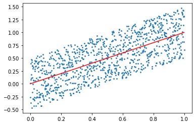
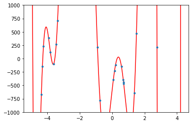
Today I started my linear algebra class by motivating the determinant using a little bit of history and applications. In particular I talked about determinant appearing in the change of variables in integration of multivariate functions in calculus:Then after the class I noticed that my picture of what happens when we linearize the image wasn’t very clear as I had drawn it. So I decided to take a look at an actual example. The following code takes a function that maps to and draws three regions:

• the unit cube in blue,
• the image of the unit cube under in red, and
• the linearization of the image by Jacobian of at the origin

def show_linearization(f,n=100):
    # f is a function that maps R^2 to R^2 for example
    # f(x,y) = ((x^2+2*(x+2)*(y+1))/4-1,y^2-(x+1)*y)
    # The output is three areas:
        # the unit cube
        # the image of unit cube under f
        # the linearization of the image using the Jacobian of f at (0,0)
    
    var('x y')
    A = jacobian(f,(x,y))(0,0)
    p = f(0,0)
    domxy = []
    imgxy = []
    jacxy = []
    for i in range(n+1):
        for j in range(n+1):
            domxy.append((i/n,j/n))
            imgxy.append(f(i/n,j/n))
            jacxy.append(p+A*vector([i/n,j/n]))
            
    P = points(domxy,color="blue",aspect_ratio=1, alpha = .3)
    Q = points(imgxy,color="red",aspect_ratio=1, alpha = .3)
    R = points(jacxy,color="green",aspect_ratio=1, alpha = .3)
    
    (P+Q+R).show()

Here is a sample run:

f(x,y) = ((x^2+2*(x+2)*(y+1))/4-1,y^2-(x+1)*y)
show_linearization(f)

and the output is:

I chose the function in a way that for simplicity. Here it is on sage cell server for you to play around with it: link.

What do you think? Any suggestions or comments?

Step-by-step reduction

One of the things that I always tell my students is to check their solutions when they are done solving a problem. That by itself can mean several things, depending on what the problems is. Of course after solving a system of linear equations, one would plug in the solutions into the original system of equations to see if they are satisfied. The harder part is to come up with a way to check if you’ve done the row-reduction correctly or not. One can easily use Sage to see if the reduced row echelon form is computed correctly. If A is your matrix, just input A.rref() to find the reduced row echelon form of it.

But still sometimes in the case that the answer is wrong, one might get frustrated by not trying to figure out in which step they’ve made an error, or sometimes they might just get stuck. Considering that row-reduction is a time consuming process, it is plausible to assume that some one can easily give up after a few tries. I have found this nice code in Sage that shows step-by-step Gauss-Jordan elimination process, and actually tells you what to do in each step, from here. Then I did a little bit of customization on it. Here is the final version:

# Naive Gaussian reduction
def gauss_method(MATRIX,rescale_leading_entry='Last'):
    """Describe the reduction to echelon form of the given matrix of rationals.

    MATRIX  matrix of rationals   e.g., M = matrix(QQ, [[..], [..], ..])
    rescale_leading_entry='First' make the leading entries to 1's while doing Gaussisan ellimination
    rescale_leading_entry='Last' (Default) make the leading entries to 1's while reducing

    Returns: reduced form.  Side effect: prints steps of reduction.

    """
    M = copy(MATRIX)
    num_rows=M.nrows()
    num_cols=M.ncols()
    show(M.apply_map(lambda t:t.full_simplify()))

    col = 0   # all cols before this are already done
    for row in range(0,num_rows): 
        # ?Need to swap in a nonzero entry from below
        while (col < num_cols
               and M[row][col] == 0): 
            for i in M.nonzero_positions_in_column(col):
                if i > row:
                    print " swap row",row+1,"with row",i+1
                    M.swap_rows(row,i)
                    show(M.apply_map(lambda t:t.full_simplify()))
                    break     
            else:
                col += 1

        if col >= num_cols:
            break

        # Now guaranteed M[row][col] != 0
        if (rescale_leading_entry == 'First'
           and M[row][col] != 1):
            print " take",1/M[row][col],"times row",row+1
            M.rescale_row(row,1/M[row][col])
            show(M.apply_map(lambda t:t.full_simplify()))
            
        for changed_row in range(row+1,num_rows):
            if M[changed_row][col] != 0:
                factor = -1*M[changed_row][col]/M[row][col]
                print " take",factor,"times row",row+1,"plus row",changed_row+1 
                M.add_multiple_of_row(changed_row,row,factor)
                show(M.apply_map(lambda t:t.full_simplify()))
        col +=1

    print "Above is a row echelon form, let's keep cruising to get the reduced row echelon form:\n"
    
    for i in range(num_rows):
        row = num_rows-i-1
        if M[row] != 0:
            for col in range(num_cols):
                if M[row,col] != 0:
                    if M[row,col] != 1:
                        print " take",1/M[row][col],"times row",row+1
                        M.rescale_row(row,1/M[row][col])
                        show(M.apply_map(lambda t:t.full_simplify()))
                    break

            for changed_row in range(row):
                factor = -1 * M[row-1-changed_row,col]
                if factor != 0:
                    print " take", factor,"times row", row+1, "plus row", row-1-changed_row+1
                    M.add_multiple_of_row(row-1-changed_row,row,factor)
                    show(M.apply_map(lambda t:t.full_simplify()))
    return(M.apply_map(lambda t:t.full_simplify()))

And here is a sample run:

M = matrix(SR,[[3,-1,4,6],[0,1,8,0],[-2,1,0,-4]])
gauss_method(M,rescale_leading_entry='First')

And the output looks like this:

Click here to run it in the sage cell server. Note that the code is implemented to work over rational field since it is being used for pedagogical reasons.

In the comments Jason Grout has added an interactive implementation of the first part of the code:

# Naive Gaussian reduction
@interact
def gauss_method(M=random_matrix(QQ,4,algorithm='echelonizable',rank=3),rescale_leading_entry=False):
    """Describe the reduction to echelon form of the given matrix of rationals.

    M  matrix of rationals   e.g., M = matrix(QQ, [[..], [..], ..])
    rescale_leading_entry=False  boolean  make the leading entries to 1's

    Returns: None.  Side effect: M is reduced.  Note: this is echelon form, 
    not reduced echelon form; this routine does not end the same way as does 
    M.echelon_form().

    """
    num_rows=M.nrows()
    num_cols=M.ncols()
    print M    

    col = 0   # all cols before this are already done
    for row in range(0,num_rows): 
        # ?Need to swap in a nonzero entry from below
        while (col < num_cols                and M[row][col] == 0):              for i in M.nonzero_positions_in_column(col):                 if i > row:
                    print " swap row",row+1,"with row",i+1
                    M.swap_rows(row,i)
                    print M
                    break     
            else:
                col += 1

        if col >= num_cols:
            break

        # Now guaranteed M[row][col] != 0
        if (rescale_leading_entry
           and M[row][col] != 1):
            print " take",1/M[row][col],"times row",row+1
            M.rescale_row(row,1/M[row][col])
            print M
        change_flag=False
        for changed_row in range(row+1,num_rows):
            if M[changed_row][col] != 0:
                change_flag=True
                factor=-1*M[changed_row][col]/M[row][col]
                print " take",factor,"times row",row+1,"plus row",changed_row+1 
                M.add_multiple_of_row(changed_row,row,factor)
        if change_flag:
            print M
        col +=1

One of the uses of this can be to find the inverse of a matrix step by step. For example:

var('a b c d')
A = matrix([[a,b],[c,d]])
R = gauss_method(A.augment(identity_matrix(A.ncols()),subdivide=True))

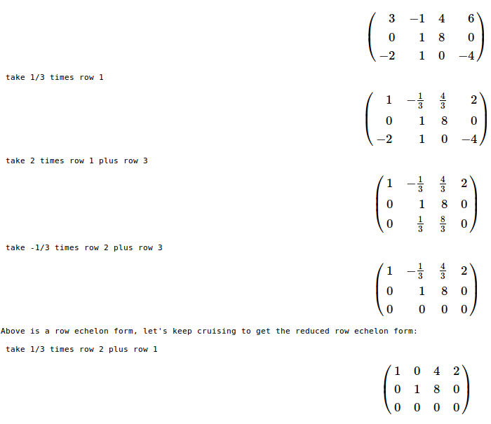
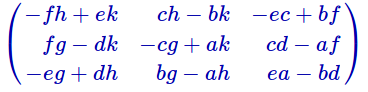
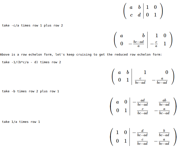
will give you: Or you can run it for a generic matrix of size 3 (for some reason it didn’t factor i, so I used letter k instead:)

var('a b c d e f g h i j k l m n o p q r s t u v w x y z')
A = matrix([[a,b,c],[d,e,f],[g,h,k]])
R = gauss_method(A.augment(identity_matrix(A.ncols()),subdivide=True))

The steps are too long, so I’m not going to include a snapshot, if you are interested look at the steps here. But you can check out only the final result by

view(R.subdivision(0,1))

which will give you And to check if the denominators and the determinant of the matrix have any relations with each other you can multiply by the determinant and simplify:

view((det(A)*R.subdivision(0,1)).apply_map(lambda t:t.full_simplify()))

to get

Do you think this can help students?